Abstract
Background Matching is a popular technique for improving covariate balance in observational data. Because the method has been fully implemented in a variety of software packages, the inner workings are not necessarily clear to the analyst. Recent criticisms of Propensity Score Matching, in particular, have highlighted a need to give more insight and clarity to the black box that is Matching.
Aim We set out to develop an interactive space where users can understand matching algorithms and compare results based on different user specifications. We wanted users to be able to compare methods of matching but more importantly, to compare the underlying settings that can be used to generate the matches, including the selection of matching covariates, the order the matches were conducted in, and whether or not replacement was used.
Solution WhatsMatching is an interactive Shiny app that allows users to simulate data and watch matching algorithms dynamically unfold. It provides options for using the Propensity Score Distance and the Mahalanobis Distance to match on and includes all the settings laid out in the aim.
Dissemination The Golem framework has been the underpinning guide for development. This has allowed the provision of an installable R package, a Shiny app deployed on shinyapps.io, and all documentation and vignettes on a package website. All code is opensource and available on GitHub.
Overview
The problem and promise of observational data
Estimating the causal effect of a treatment or intervention is a core task of health data science. Randomised control trials (RCTs) are the gold standard study design for estimating treatment effects, but in many contexts RCTs are not feasible, for logistic or ethical reasons. As a result, researchers often turn to observational data to address causal research aims. These data are not ideal because there is no control over who receives the treatment or exposure of interest and who does not, introducing potential selection and confounding biases. Nonetheless, observational data are a useful asset, being relatively cheap and easy to access, and for exposures that cannot ethically be manipulated, they offer the only possibility of investigating research questions of interest.3,4,11
Approaches to obtaining valid causal inferences from observational data
It is still possible to obtain valid estimates of causal effects from observational data, provided the limitations of the data are addressed in the analysis. Many methodological approaches to address confounding bias have been proposed over the years, including stratification, regression adjustment, matching, applications of the propensity score and g-computation methods.3,8 The primary aim of these methods is to reduce bias in the estimation of the casual effect, especially confounding, by balancing the distribution of confounding variables in the treated and control groups.7,12
Matching methods
Matching is a general pre-processing technique used to improve causal estimates from observational data by matching treated individuals to untreated individuals (controls) with the same or similar background characteristics. The objective of matching is to balance key background characteristics in the treated and control groups. In a RCT this balance is achieved through randomisation; the intuitive appeal of matching is as a simple way to find a RCT “hidden” in an observational dataset.4
The most basic form of matching is exact matching. This is where treated and control groups have their key characteristics matched exactly. For example, if matching is done on age and sex, a treated 45 year old male will be matched with an untreated 45 year old male. When there are a small number of matching variables and the pool of potential matches is large it can be possible to match each treated individual to a control with the exact same characteristics, leading to a perfectly balanced dataset. However, using exact matching is often infeasible in practice, especially if there are numerous matching variables and/or a small pool of potential matches.
One alternative to exact matching is coarsened exact matching. Under this approach, matching variables are temporarily coarsened, for example age measured in years might be recoded to 10-year age bands. The coarsened variables are then used to undertake exact matching, and once the balanced dataset is found the analysis can proceed with the original uncoarsened data.
A second alternative to exact matching is distance-based matching. Distance-based matching proceeds by matching treated and untreated individuals based on some distance metric that quantifies the similarity between each pair of individuals in the dataset. Perhaps the most widely used distance metric is the propensity score, defined as the probability of an individual receiving the treatment.11 Another possible distance metric is the Mahalanobis distance, which is analogous to a multivariate Euclidean distance.4
The advantage of both the propensity score and the Mahalanobis distance metrics is that the multidimensional covariate space is reduced to a single dimension: matching can be undertaken on the univariate distance measure rather than attempting to match each individual covariate. The covariates that define the distance metric are balanced between the treated and control groups, on average, in the resulting matched dataset.
The propensity score
Perhaps one of the most popular and enduring family of techniques for estimating causal effects from observational data revolve around the propensity score. Rosenbaum and Rubin (1983) defined the propensity score as the “conditional probability of assignment to a particular treatment given a vector of observed covariates”.11 Mathematically, this can be expressed as \(e(x_i) = pr(Z_i=1|x)\) where \(e(x_i)\) is the propensity score, \(Z\) is the treatment variable, \(x\) is a vector of covariates, and \(i\) represents an individual.
In most cases, the propensity score is estimated from available data using a simple logistic regression on a binary treatment assignment indicator. The logistic regression formula may take the form of \(t \sim x_1 + ... + x_n\) where \(t\) is a binary indicator of whether or not the individual received treatment and \(x_1 \ldots x_n\) represent \(n\) observed covariates that help to predict the treatment outcome. Although logistic regression is widely used for this step, the estimation method is at the discretion of the analyst and more flexible models can perform well.6
Once estimated, the propensity score can be incorporated into the data analysis in multiple ways. This includes matching, weighting and stratification (AKA subclassification). All three applications are briefly described below. Matching is the the primary focus of the WhatsMatching app, however the app also allows comparisons in estimates based on all three approaches.
Applications of propensity scores – matching, weighting and stratification
Matching
A common application of the propensity score is as a distance metric in distance-based matching. The distance between two individuals is defined as the absolute difference in their propensity scores \(|e(x_1) - e(x_0)|\). Treated individuals are matched to untreated individuals with similar propensity scores, and in doing so the covariates that are used in the propensity score estimation should be balanced on average in the treated and control groups.
Many packages in R that perform matching analysis also
automate the process of estimating the propensity score. Once the
probabilities have been calculated then treated units are paired with
control units that have the same or similar probability of
treatment.
It is important to note that estimated effects generally correspond to the average treatment effect on the treated (ATT) when using matching methods. This makes sense intuitively as matching effectively removes individuals from the data that could not be considered both treated and untreated. This is referred to as strongly ignorable treatment assignment and is a key assumption for providing unbiased estimates with the propensity score.
Weighting
Weighting with the propensity score differs from matching as no units are pruned from the dataset. This is an advantage over matching in the sense that all data can remain in the analysis, giving the opportunity to calculate the average treatment effect on all units (ATE), as opposed to the ATT.
The formulas for weighting vary depending on the method you want to
employ. The data being analysed, by virtue of its source, may be more
appropriately analysed for the ATT and not the ATE. The formulas for
these weights are:
\[ATE,
w(W,x)=\frac{W}{\hat{e}(x)}+\frac{1-W}{1-\hat{e}(x)}\]
\[ATT,
w(W,x)=W+(1-W)\frac{\hat{e}(x)}{1-\hat{e}(x)}\]
where \(\hat{e}(x)\) indicates the
estimated propensity score conditional on observed \(x\) covariates.1,11
Stratification (aka Subclassification)
The stratification method varies from matching and weighting in that it relies on the use of the propensity score to group units into quantiles. Once the number of groups has been established, the literature suggests this is between five and ten depending on the size of the dataset,7 the treatment effect is estimated across the groups and then averaged to give a mean difference ATE.1,11
The Mahalanobis distance
The Mahalanobis Distance was developed by Prasanta Chandra Mahalanobis in 1936 as a means of comparing skulls based on their measurements. It’s normal application calculates how many standard deviations a point is from the mean of the specified variables and can give a good indication of outliers in a group.9,10 In matching, the application is similar but not quite the same. Instead of using the mean as a comparator, each treated unit is compared, pair-wise, with each of the units in the control group.4
The pair-wise Mahalanobis Distance is calculated by \(D_{ij} = \sqrt{(X_i−X_j)S^{−1}(X_i−X_j)}\) where \(D_{ij}\) is the pair-wise Mahalanobis distance, \(X_i\) and \(X_j\) represent the matrix of covariates for the treated and control groups and \(S^{-1}\) is the covariance matrix.4 Similar to the Propensity Score, the Mahalanobis Distance reduces a multidimensional space to a single value representing the distance between units. A key difference in understanding how the matching works between these methods is understanding that the Mahalanobis distance is the measured distance between units whereas the Propensity Score distance is the difference in the probabilities of treated and untreated units.
It should be further noted that individual units have their own propensity score (or probability of being treated) however, they do not have a Mahalanobis value assigned to them. The value from the Mahalanobis distance is between the units. This is a fundamental difference in the way the matching occurs because, while the true values of the covariates have been used to determine the probability of treatment, the propensity score is blind to the real data.
Gaps in Understanding
The propensity score matching process appears to be straight forward and require little effort to implement, which is reflected in its ubiquitous use. However, as King and Neilsen4 point out, there are many situations where the use of the propensity score for matching may not be suitable. Their 2019 paper gives many insights into the use of the propensity score and why other methods, like coarsened exact matching or distance-based matching with the Mahalanobis distance, may be better choices. While some of the explanations do make intuitive sense it can be difficult to decipher the practical application and implications of the advice.
Matching Settings
While the choice in the distance used for matching can obviously make a difference to how units are paired, it is less clear what the implications of changing any of the many settings that are available in order to “optimise” the matches. The settings that we will discuss further include order, replacement, and calliper adjustment.
Order
Order refers to the order the matches are specified in the matching
algorithm. In the MatchIt package,2 users are only able to specify
an order for specific methods. In particular, propensity score methods
can control the order of the matching as they are a vector of
probabilities that aligns with the data. The default for the order is
data, otherwise ordering can be conducted by smallest,
largest, or random. The resultant ordering is as
follows:
data - the order supplied by the dataframe
smallest - matches occur starting with the smallest propensity score first
largest - matches occur starting with the largest propensity score first
random - matches occur randomly
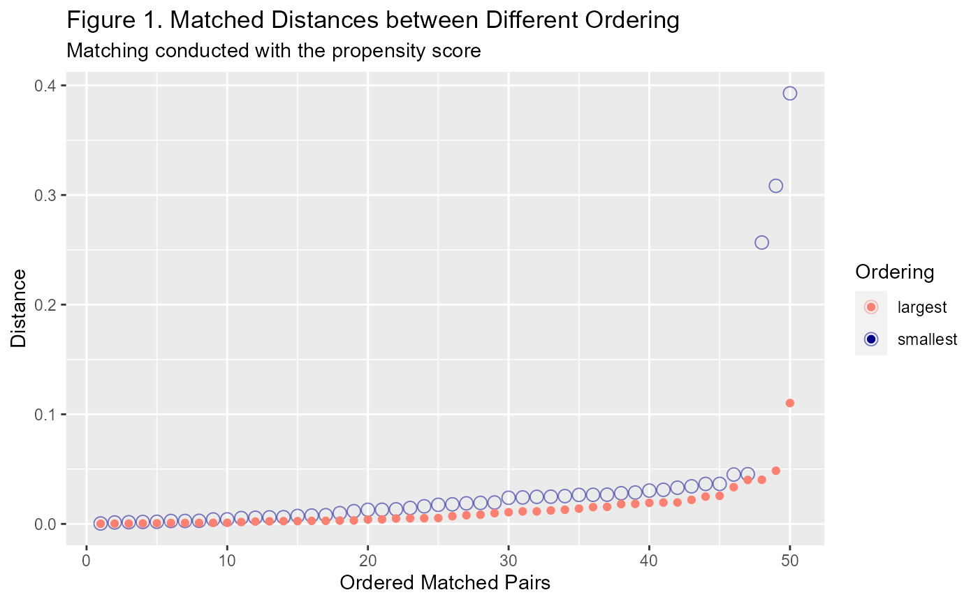
Why does ordering make a difference? Well, when you have lots of treated units close to a single untreated unit, only one of the treated units will be able to match with it. Once that untreated unit has been used, the other treated units will have to look further afield. Generally this does not impact the matches at first but towards the end of the iterative process it can. See Figure 1 below to see the difference between the distances generated by using the smallest ordering vs the largest ordering.
Replacement
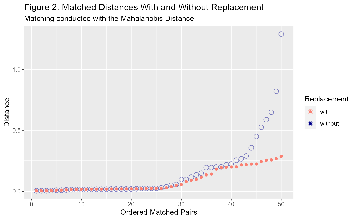
Replacement is a setting that controls whether an untreated unit can be reused. It is applicable for both MDM and PSM and other forms of matching where units are paired (as opposed to grouped). Using replacement means that you may be able to improve your covariate balance because the treated unit will be matched with the closest untreated unit, irrespective of the order. In other words, ordering is redundant when replacement is used.
It is important, however, that appropriate steps are taken to account for an untreated unit being matched multiple times. There are two main ways this can be dealt with: 1. include duplicates of the untreated data in the matched dataset; 2. apply appropriate weighting to include when estimating the treatment effect.
Calliper Adjustment
The callipers setting can be used to avoid matching units that are considered too far apart, based on some distance threshold. The implications of using this setting in practice is not particularly clear. If you cast your eyes back to Figures 1 and 2, you can see that there are units towards the end that are further apart than the rest of the group. The calliper setting seeks to remove those outliers with the intention of improving covariate balance.
The propensity score paradox
King and Neilsen4 presented a paradox that arises when using the propensity score for matching. They were able to demonstrate that, when compared to other matching distances like the Mahalanobis distance, matching on the propensity score only approximated a randomised experiment as opposed to a more efficient fully blocked experiment.
As the matching algorithm proceeds, unmatched observations are pruned from the dataset. Initially, this reduces the imbalance between the treated and untreated groups with corresponding improvements to the estimated treatment effect. However, after a certain threshold is reached, further pruning the dataset starts to result in more biased estimates of the treatment effect. This is the PSM paradox.
The authors postulated that this made matching on the propensity score inferior and were able to demonstrate this concept visually but were unable to provide mathematical proofs of the implications for real data.
Model Dependence
Another issue that can arise generally with causal inference, but then also specifically with matching, is model dependence. This is essentially where the model selection still plays a large role in predicting the estimate of the treatment effect. This is a problem because that probably means that matching has not fixed the issue of confounding and now selection bias needs to be managed as well.
Statement of research aim
Any sufficiently advanced technology is indistinguishable from magic.
–Author C. Clarke
The flexibility and convenience of distance-based matching approaches have led to numerous software implementations and widespread use across several quantitative disciplines. This is perhaps especially true of propensity score matching, a modern workhorse of causal inference. However, as with any sufficiently advanced technology, the complexity of distance-based matching can be lost on the end user. The many subjective decisions can be absorbed into the black box of a software function, with nicely matched datasets appearing, as if by magic, at the other end.
The aim of this research is to explore some basic matching methodology and provide an interactive and educational space for people who want to better understand matching methods. I will crack open the propensity score matching algorithm, allowing users to visualise matching algorithms as they dynamically unfold, and compare results under different combinations of user settings.
The resulting space is provided as a publicly available, interactive Shiny App and supported by a website and R package stored on Github. This will allow students to experiment with different matching methods and more experienced users to simulate their own matching experiments in the R environment.
Interactive applications to support learning
Learning by doing has been demonstrated to significantly improve learning when properly scaffolded, especially as part of Massive Open Online Courses (MOOCs), which are a key component of the modern educational tool kit in tertiary settings5.
RStudio supports the implementation of learnr packages that are used to provide self guided, tutorial style experiences for users. This option has had wider uptake in the tech savvy academic community. There has also been recent growth in the use of interactive learning websites like Kahn Academy. In this environment users are able to access scaffolded learning through theoretical concepts coupled with practical applications. As noted above, this has been found to be an effective method for providing education.
The space for app development
This project is aimed at the development of an educational tool where users can build an intuitive understanding of matching methods and compare different methods as discussed above. Using this educational tool, students will be able to generate data and visualise the matching process as it unfolds. Users will also be able to compare the performance of matching, with different degrees of pruning, to the weighting and stratification applications of the propensity score that don’t involve pruning, and to matching approaches using the alternative Mahalanobis distance.
Currently, there is no available platforms to compare matching methods interactively. The purpose of the app is to provide educational support and the ability for users to play with and visualise how matching occurs. In addition, this app has been developed as a package which contains easy to use functions that are available to more advanced users who may want to investigate beyond the constrains of the Shiny App.